Machine Learning Training from Scratch: Loss, Gradients, and Overfitting

Most beginner ML code hides the only thing you really need to understand: why the weights move. loss.backward() looks like a magic spell until you have derived one gradient by hand and watched it update a parameter.

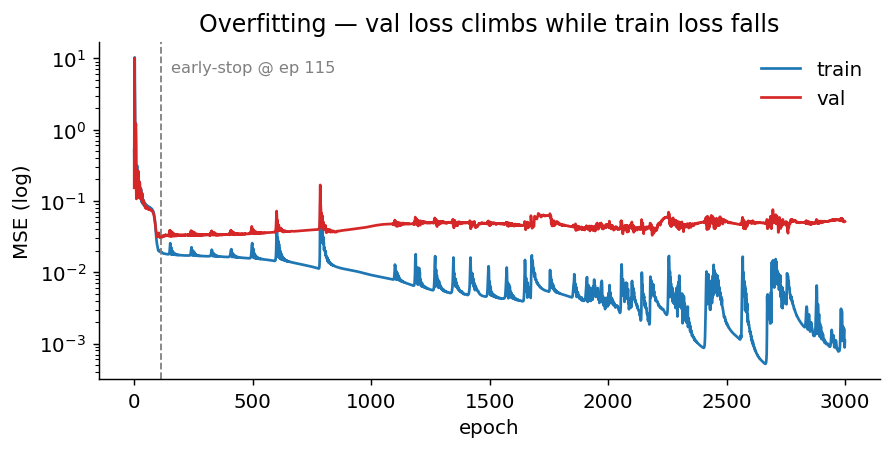
This tutorial makes that update visible. We start with one-parameter regression, write the training loop in NumPy, then let PyTorch autograd do the same job. The second half is the failure mode every useful model eventually hits: training loss keeps falling while validation loss turns around and climbs.

for xb, yb in train_loader:
    pred = model(xb)
    loss = loss_fn(pred, yb)
    optimizer.zero_grad()
    loss.backward()
    optimizer.step()

Try it before you read it

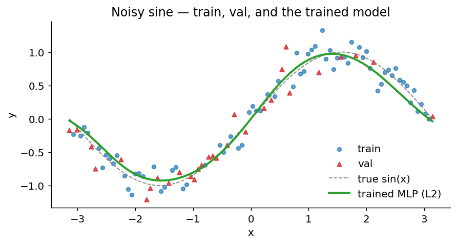
Drag the slider, hit play, and watch a deliberately over-large network follow the data — past the point where it starts memorising the noise.

The gradient by hand

Before writing code, it is useful to see one update without autograd. Suppose the model is a line,

[ \hat{y} = w x + b. ]

and the loss is mean squared error,

[ \mathcal{L}(w,b) = \frac{1}{N}\sum_{i=1}^{N}(\hat{y}i-y_i)^2 = \frac{1}{N}\sum{i=1}^{N}(w x_i+b-y_i)^2 . ]

Let (e_i = \hat{y}_i-y_i). The chain rule gives

[ \frac{\partial \mathcal{L}}{\partial w} = \frac{2}{N}\sum_{i=1}^{N} e_i x_i, \qquad \frac{\partial \mathcal{L}}{\partial b} = \frac{2}{N}\sum_{i=1}^{N} e_i . ]

Gradient descent then moves in the opposite direction to the gradient:

[ w \leftarrow w-\alpha\frac{\partial\mathcal{L}}{\partial w}, \qquad b \leftarrow b-\alpha\frac{\partial\mathcal{L}}{\partial b}. ]

The learning rate (\alpha) controls the step size. If it is too small, training crawls; if it is too large, the update can jump over the minimum.

From the derivative to code

In NumPy, the forward pass and the two derivatives have to be written explicitly:

for epoch in range(100):
    y_pred = w * x + b

    error = y_pred - y
    loss = (error ** 2).mean()

    grad_w = 2 * (error * x).mean()
    grad_b = 2 * error.mean()

    w -= learning_rate * grad_w
    b -= learning_rate * grad_b

For a deep network, writing every derivative by hand is not practical. PyTorch records the forward computation and applies the chain rule during loss.backward():

for epoch in range(100):
    y_pred = model(x)
    loss = loss_fn(y_pred, y)

    optimizer.zero_grad()
    loss.backward()
    optimizer.step()

That is the same mathematical update, but PyTorch computes the gradients for all trainable parameters automatically.

Video explainers: layer forward pass

Watch this before continuing if the forward pass still feels abstract. The page loads only the recording that matches your current light or dark theme.

Open the YouTube channel →

Try the layer yourself

This is the scalar version of a neural-network layer. Change the input, weight, bias, and activation. The page computes the pre-activation value (z = wx + b), then applies the activation function to produce the layer output.

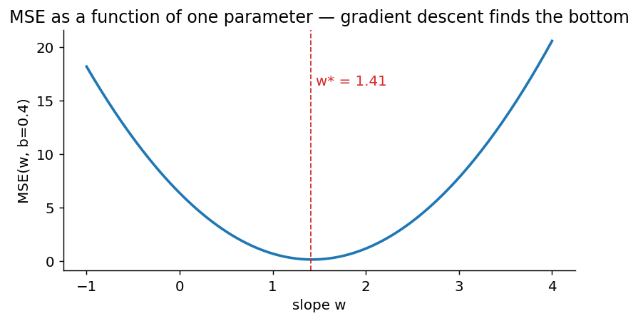
The loss landscape

For a linear model ŷ = w·x + b with mean-squared-error loss, fixing b and sweeping w traces out a parabola. The minimum is the best slope. Gradient descent’s job is to slide down it.

Reading a loss curve

If you take only one thing from this tutorial, take this: a loss curve with only the train line is a lie. Train loss falling means the optimiser is doing its job. Val loss is the only readout that tells you whether the model is learning or just memorising.

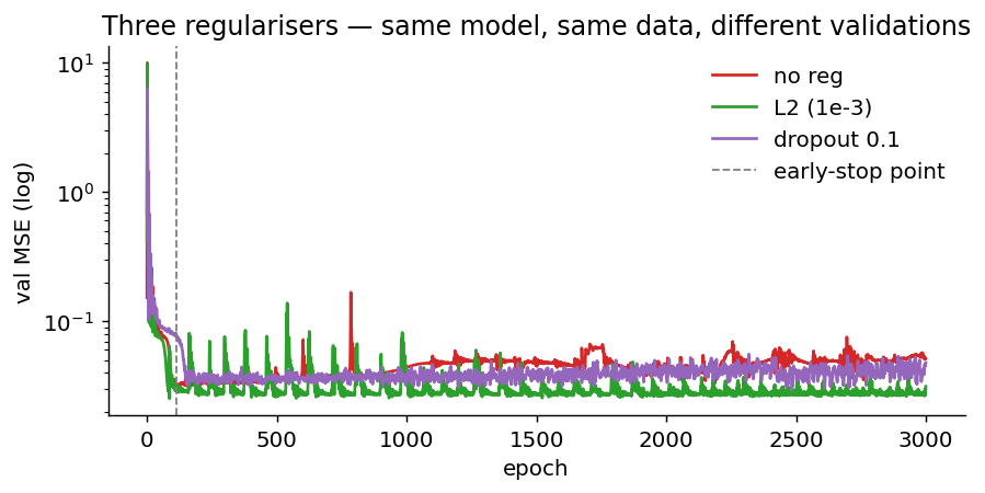
Three knobs that fix overfitting

Watch the model find the function

What’s in here

• The MSE loss landscape, drawn as a 1-D slice
• The gradient of MSE, derived by hand
• A NumPy training loop, then the same loop in PyTorch using autograd
• The five-line training pattern (forward → loss → zero → backward → step) that every PyTorch model in this series uses
• A deliberate overfit on a 5-hidden-layer, 128-wide MLP
• Three regularisers — early stopping, L2 weight decay, dropout — compared
• torch.save / torch.load patterns that decouple weights from code

Prerequisites

• Python (you’ve written a for loop)
• NumPy arrays
• High-school calculus (one chain rule)

Next

• 02 — scikit-learn intro — the classical tabular-ML workflow any PyTorch training loop also needs.
• 05 — physics-informed neural networks — what changes when the loss function knows physics.

References

1. Srivastava, Hinton et al. (2014). Dropout. JMLR 15(56). JMLR
2. Kingma & Ba (2015). Adam: A method for stochastic optimization. arXiv:1412.6980
3. Goodfellow, Bengio & Courville (2016). Deep Learning (MIT Press), chs 7–8. deeplearningbook.org
4. Karpathy (2022). The spelled-out intro to neural networks and backpropagation. karpathy.ai