scikit-learn Regression Tutorial: Explore, Fit, Evaluate, Diagnose

The mistake in beginner scikit-learn is not usually the .fit() call. It is trusting the first number that looks good. A model can draw a nice line and still fail systematically on the held-out data.

The day-to-day API is tiny: instantiate a model, call .fit, call .predict. Everything else is choosing which model, which features, and which numbers to trust when evaluating it.

from sklearn.metrics import root_mean_squared_error, r2_score

model = LinearRegression()
model.fit(X_train, y_train)
pred = model.predict(X_test)
rmse = root_mean_squared_error(y_test, pred)
r2 = r2_score(y_test, pred)

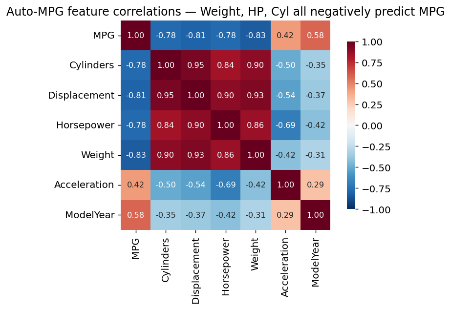
This tutorial walks the entire workflow on the UCI auto-MPG dataset — 392 cars from the 1970s and 80s — and ends with the diagnostics that turn a fit into an honest answer. We start with a single feature (Weight → MPG), then add Horsepower and Cylinders, and watch the metrics improve.

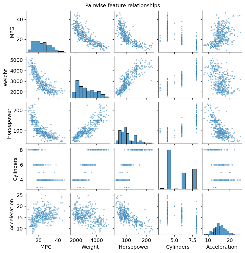
Pearson correlation heatmap of MPG, Weight, Horsepower, Cylinders, Displacement, Acceleration, ModelYear — The first plot to make on any tabular dataset. Strong negative correlations between MPG and Weight / Horsepower / Cylinders — heavier, more powerful cars use more fuel. ModelYear is positive — fuel efficiency improved through the 1980s.

Pairwise relationships

Pairplot of MPG vs Weight, Horsepower, Cylinders, Acceleration with diagonal histograms — The full pairwise plot. Weight and Horsepower are highly collinear (which will matter when we interpret the multivariate coefficients).

The single-feature fit

Three lines and you have a linear regressor: LinearRegression(), .fit(X, y), .predict(X_test). The pattern is the same for every model in sklearn.

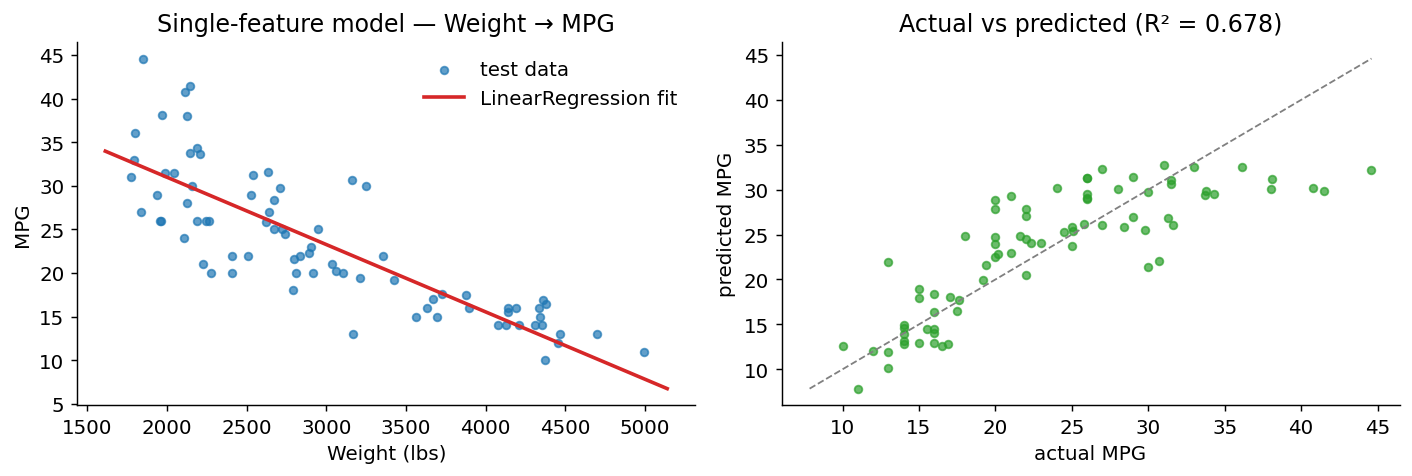
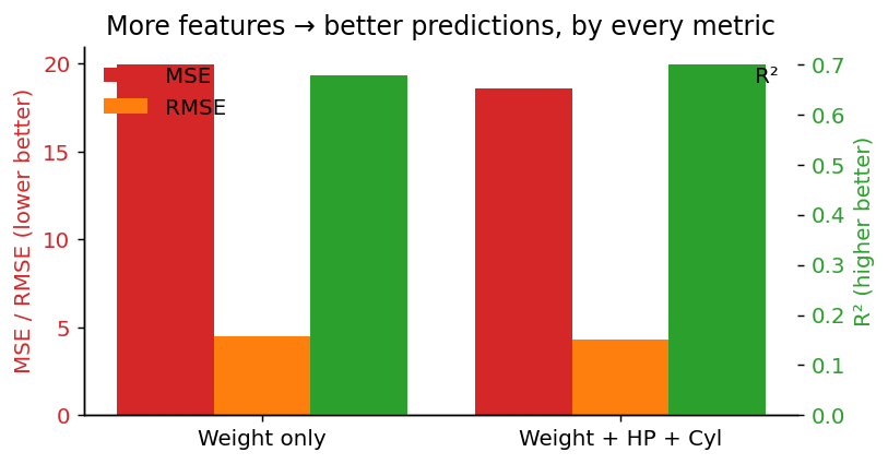
Weight vs MPG scatter with regression line on the left, actual vs predicted MPG on the right — Left: Weight → MPG with the fitted line. Right: actual vs predicted on the held-out test set. Systematic deviations from the diagonal are the first sign of a bad model.

Weight alone explains 67.8 % of the variance in MPG (R² = 0.678, RMSE = 4.47). Already decent for one column.

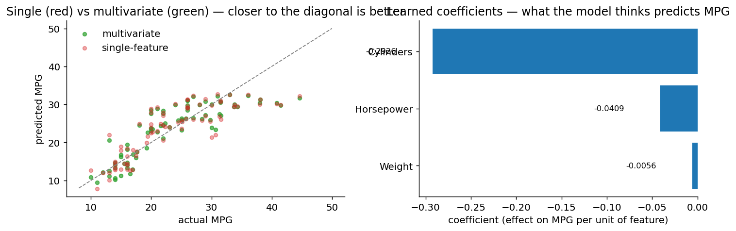
Adding more features

Same workflow, more columns in X. Going to Weight + Horsepower + Cylinders improves R² to 0.701 (RMSE 4.31). Modest gain because Weight is already capturing most of the predictable variance — Horsepower and Cylinders are heavily correlated with it.

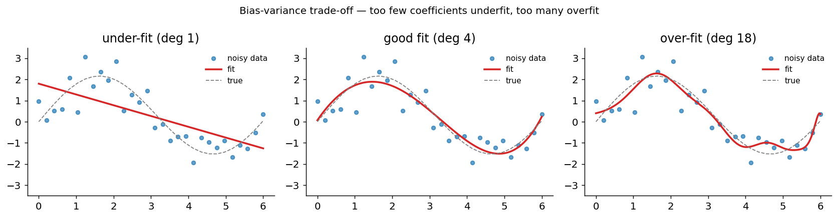
Single vs multivariate predicted-vs-actual scatter on left, learned coefficients bar chart on right — Left: the multivariate model's predictions cluster closer to the diagonal. Right: the three learned coefficients. The Weight coefficient is small but the feature spans thousands of pounds; the Cylinders coefficient looks large but the feature only spans 3-8.

Side-by-side bars for MSE, RMSE, and R² for the single vs multivariate model — Every metric moves the right direction once you add the other features.

The bias-variance trade-off

A linear model with one feature cannot capture curvature — it underfits. A polynomial regression with too many terms memorises the noise — it overfits. The right answer lies between. Every ML problem has some version of this picture; it is the most important intuition to internalise early.

Three panels: underfit linear, good polynomial fit, and overfit high-degree polynomial on the same noisy curve — Same noisy synthetic curve, three polynomial-regression fits. Degree 1 underfits; degree 18 follows the noise; degree 4 is right.

What’s in here

The full load → explore → split → fit → predict → evaluate workflow
Correlation heatmap + pairplot as your two first plots, always
LinearRegression, train_test_split, MSE / RMSE / R²
Single-feature vs multi-feature regression on the same data
Reading coefficients carefully when features are collinear
The bias-variance trade-off, drawn as one figure
Four open-ended exercises at the end

Prerequisites

Comfortable with pandas DataFrames
Knowing what a for loop is

03 — Introduction to Neural Networks — what changes when the model is a network and the framework is PyTorch.

References

Pedregosa et al. (2011). Scikit-learn. JMLR 12. JMLR
Quinlan, J. R. (1993). Combining instance-based and model-based learning. ICML 1993 — the auto-MPG dataset, originally from the StatLib archive. PDF
James, Witten, Hastie & Tibshirani (2021). An Introduction to Statistical Learning, 2nd ed. — chapters 3 (regression) and 5 (resampling). statlearning.com