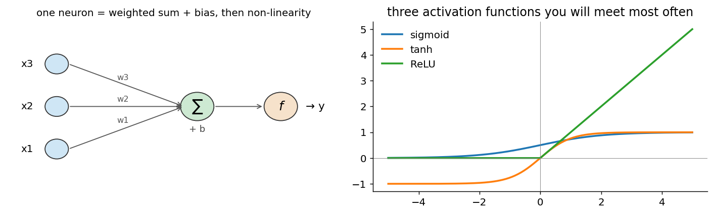
Neural Networks from One Neuron to a PyTorch MLP Classifier

The confusing part of neural networks is not the word “neural”; it is the jump from one weighted sum to a system that can learn curved decision boundaries. This tutorial keeps that jump small.

A neural network is what you get when you stack a lot of \(f(w \cdot x + b)\) neurons and let gradient descent set the weights. We build that stack one layer at a time, then use the same pattern for a classifier on the Wisconsin breast-cancer dataset (569 patients, 30 features).

model = nn.Sequential(
    nn.Linear(30, 32),
    nn.ReLU(),
    nn.Dropout(0.2),
    nn.Linear(32, 1)
)
loss = nn.BCEWithLogitsLoss()(model(x), y)

Single-neuron diagram on the left, three activation functions on the right — Left — a neuron is a weighted sum plus a bias, then a non-linearity. Right — the three activation functions you'll meet most often: sigmoid, tanh, ReLU. The choice matters.

From neuron to layer: the matrix form

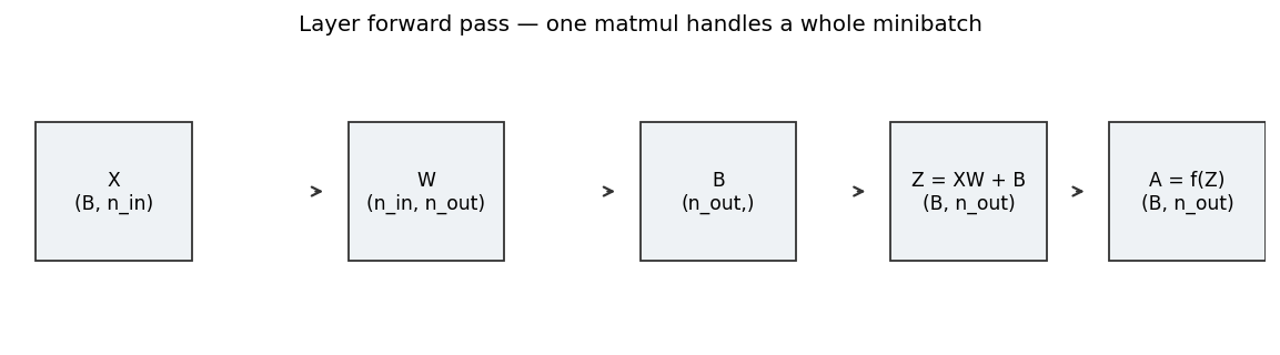
A layer is many neurons applied to the same input in parallel. Instead of computing one weighted sum at a time, a single matrix multiplication handles the whole minibatch:

\[\mathbf{Z} = \mathbf{X}\,\mathbf{W} + \mathbf{B}, \qquad \mathbf{A} = f(\mathbf{Z}).\]

\(\mathbf{X}\) is the input data.
\(\mathbf{W}\) is the weight matrix.
\(\mathbf{B}\) is the bias vector.
\(f\) is the non-linear activation function.

The activation function is what makes a stack of layers nonlinear. Without it, several linear layers collapse into one linear map, so depth alone would not add representational power.

Block diagram: X times W plus B equals Z, then activation gives A — A single matmul is enough to compute the forward pass of an entire layer for an entire minibatch.

Capacity matters — what one neuron cannot do

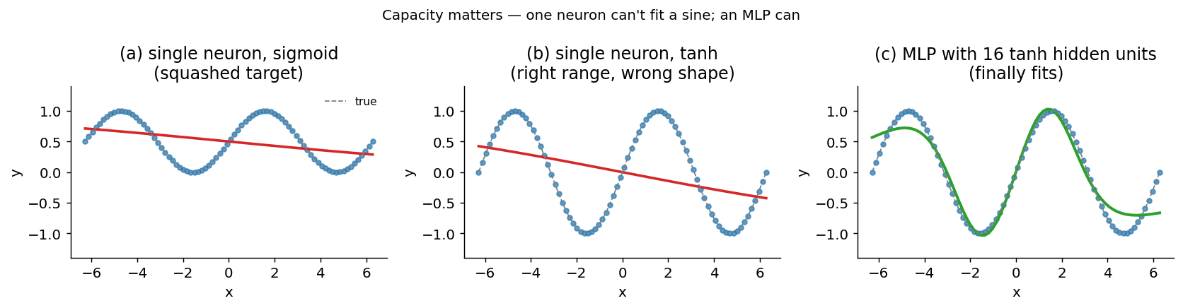
The cleanest demonstration of why we need multiple neurons is to try fitting a sine wave with one.

A single tanh neuron can choose the right output range, but its shape is still a smooth S-curve. It cannot follow a periodic function that turns up, down, and up again over the interval.

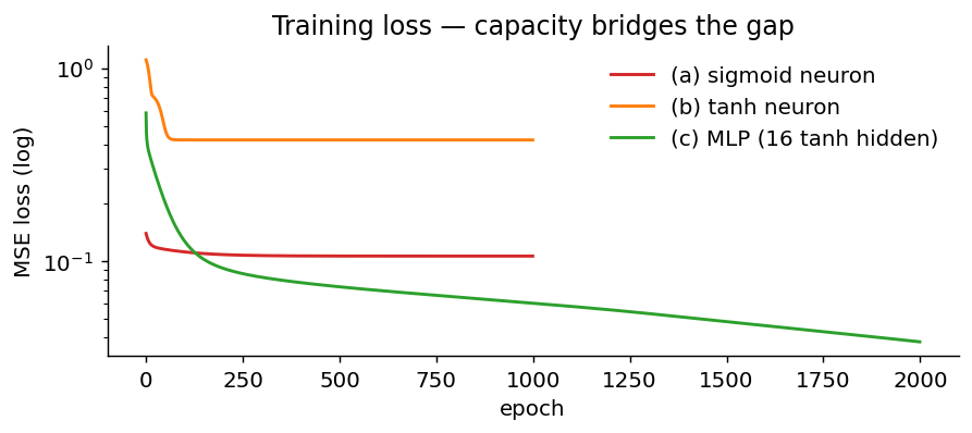
A hidden layer changes the situation. A multilayer perceptron (MLP) with one hidden layer of 16 tanh units can combine several shifted S-curves, so it fits the oscillation much more closely.

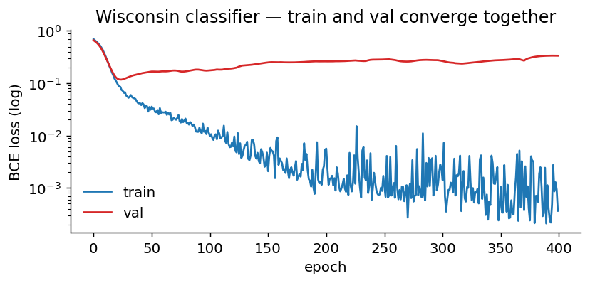
Three panels: sigmoid neuron, tanh neuron, MLP — each trying to fit a sine wave — (a) Sigmoid neuron — squashes outputs to [0, 1], misses the troughs. (b) Tanh neuron — right range, wrong shape, just a smooth ramp. (c) MLP with 16 tanh hidden units — finally fits.

Log-scale loss curves for the three models — Log-scale training loss. The MLP plateaus orders of magnitude lower than either single-neuron variant — that gap is what "model capacity" means.

Apply it — Wisconsin breast cancer

Now the MLP machinery becomes a real medical classifier. 30 numerical features (radius, texture, perimeter, area, smoothness…) per patient, binary malignant / benign label. The architecture is the same 2-hidden-layer template with dropout; the loss switches from MSE to binary cross-entropy.

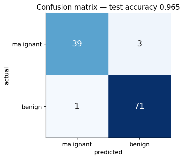
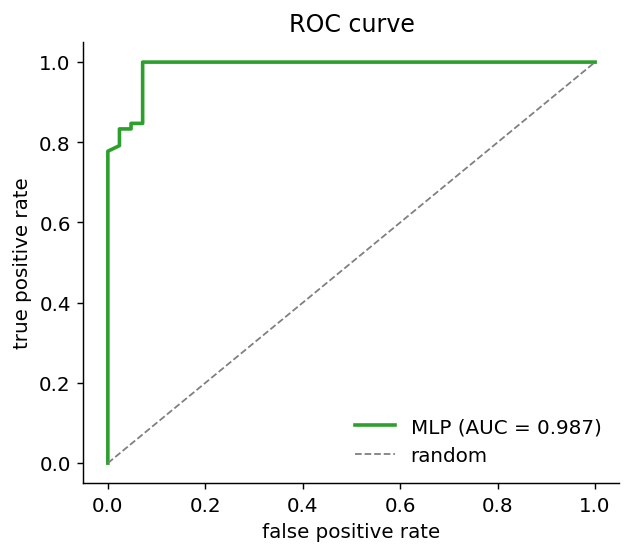
Train and val BCE loss curves across 400 epochs, both falling and staying close — Train and val BCE both fall and stay close together — dropout is doing its regularisation job.

Why accuracy alone is dishonest

A 95 %-accurate classifier that misses every cancer is worse than useless. You always want the confusion matrix (where the errors fall) and the ROC (how the trade-off between false-positives and missed-positives behaves as you sweep the decision threshold).

2x2 confusion matrix on the held-out test set — Confusion matrix on the held-out 20 % test set. Off-diagonal cells are the mistakes — the model only misses one malignant sample.

ROC curve with AUC label and random-baseline diagonal — ROC. Diagonal would be random; perfect is the top-left corner. AUC summarises the curve in one number.

What’s in here

The single neuron (f(w · x + b)), three activation choices
Matrix formulation of a layer — one matmul per minibatch
A manual gradient-descent training loop with autograd
The same model rewritten in nn.Module — verbose to terse
Activation matters — sigmoid vs tanh on a sine wave
Adding a hidden layer — when one neuron isn’t enough
Real-data application: Wisconsin breast-cancer classification
BCEWithLogitsLoss and why it beats BCE + sigmoid as two ops
Confusion matrix + ROC + AUC

Note on data ethics

The Wisconsin dataset is real but anonymised, 1995-era, and a teaching standard. Production medical-ML projects need IRB approval, calibration plots, and uncertainty quantification well beyond a confusion matrix. This tutorial is for the model and metrics, not for clinical deployment.

Prerequisites

Tutorial 01 — the training loop
Tutorial 02 — train/test splits

04 — Convolutional Neural Networks — what changes when the input is an image and you need to preserve spatial structure.

References

Wolberg & Mangasarian (1990). Multisurface method of pattern separation for medical diagnosis applied to breast cytology — the Wisconsin dataset. doi:10.1073/pnas.87.23.9193
Rumelhart, Hinton & Williams (1986). Learning representations by back-propagating errors. Nature 323. doi:10.1038/323533a0
Fawcett (2006). An introduction to ROC analysis. doi:10.1016/j.patrec.2005.10.010
Karpathy (2022). The spelled-out intro to neural networks and backpropagation. karpathy.ai