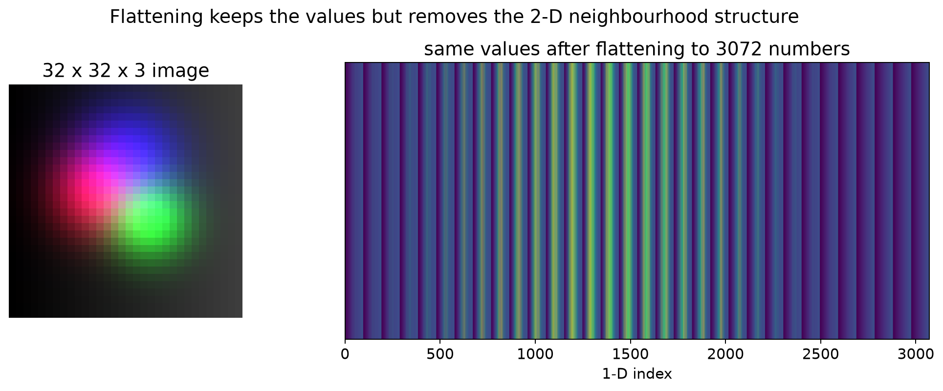
Flattening an image turns a neighbourhood into a long list. That is the first reason MLPs struggle with vision: the model has to relearn locality from scratch for every object, position, and scale.
A CNN is an MLP that shares weights spatially. Instead of one weight per input pixel, you have a 3 × 3 filter that slides across the image. That single change buys translation equivariance, parameter efficiency, and a useful inductive bias for any signal where neighbouring values are correlated: images, audio, time series, physical simulation fields. Pooling and the later architecture can then trade some of that equivariance for practical translation invariance.
conv = nn.Conv2d(in_channels=3, out_channels=32,
                 kernel_size=3, padding=1)
y = conv(x)  # [batch, 3, height, width] -> [batch, 32, height, width]
This tutorial does CNNs in three movements:
- Why we need CNNs at all — what breaks when you flatten a colour image into a 3 072-element vector and hand it to an MLP.
- The convolution operation — kernels, strides, padding, pooling. The math is small; the inductive bias is enormous.
- A trained CNN, opened up — visualising the learned filters and the feature maps they produce. CNNs are easier to interpret than modern ML literature suggests.
The runnable notebook uses sklearn’s load_digits (1 797 hand-written
8 × 8 grayscale digits) so it finishes in under a minute on CPU. This
page accompanies it with CIFAR-10 figures that were pre-rendered
locally — colour images make the lessons land harder.
CIFAR-10 — the dataset every CNN tutorial uses
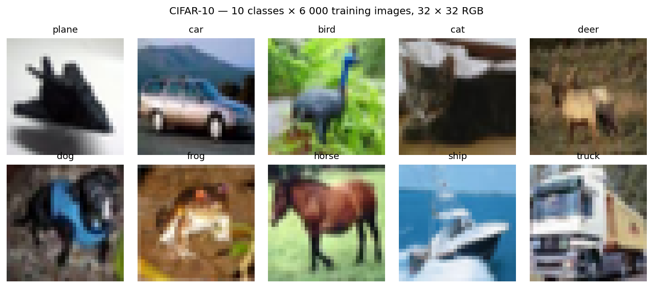
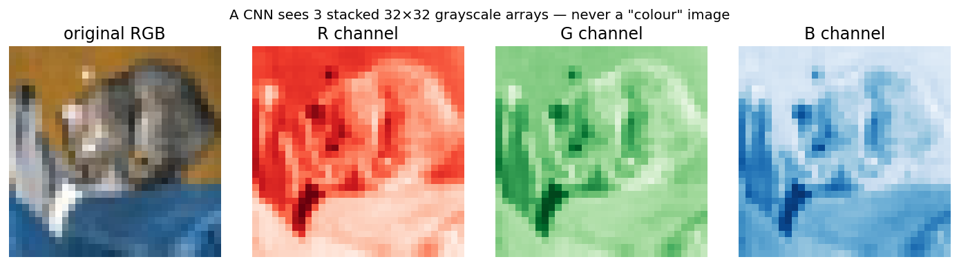
A CNN sees channels, then learns how to mix them
Channels are how a CNN handles colour: the input tensor has shape
[batch, channels, height, width] and for an RGB image, channels = 3.
The first convolutional layer receives three aligned channel maps and
each learned filter spans all three channels. So the model starts with
RGB as separate input channels, but it immediately learns cross-channel
combinations such as colour edges and opponent-colour blobs.
The killer flaw of MLPs on images — flattening
An MLP needs a 1-D input. So before you can feed an image to one, you
flatten it from [C, H, W] into a single long vector. That destroys
the very thing that makes an image an image.
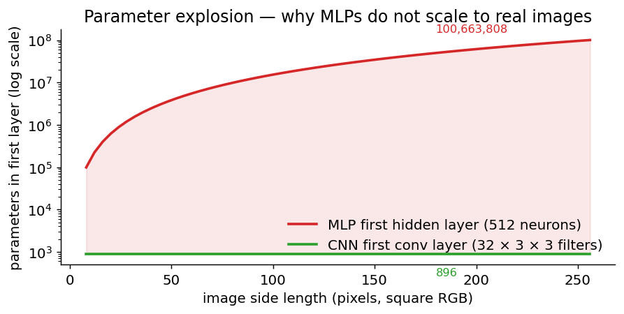
The other MLP problem — parameter explosion
For a fully-connected first hidden layer with 512 neurons:
| input image | input features | parameters in 1st hidden layer |
|---|---|---|
| 8 × 8 digits (this notebook) | 64 | 33 280 |
| 32 × 32 RGB (CIFAR) | 3 072 | 1 573 376 |
| 224 × 224 RGB (ImageNet) | 150 528 | 77 070 848 |
A CNN’s first conv layer with 32 filters of 3 × 3 × 3 has 896 parameters regardless of image size for that layer. Same weights are reused everywhere.
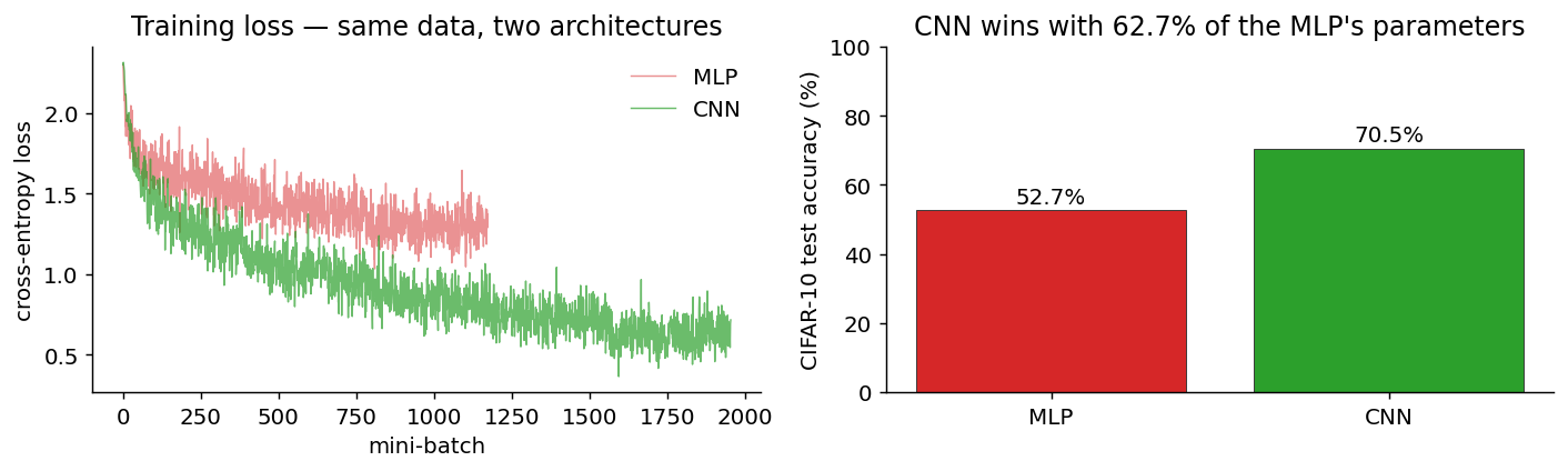
Empirical verdict: same data, two architectures
We trained both a 3-layer MLP and a 2-conv-block CNN on CIFAR-10 for a few epochs each. The MLP gets ~52 % test accuracy with 1.7 M parameters; the CNN gets ~70 % with 300 k parameters — six times smaller and significantly better.
What a convolution actually does
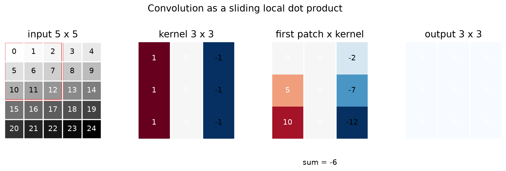
A 2-D convolution is a local weighted sum:
\[\text{output}(i, j) = \sum_m \sum_n \text{input}(i + m, j + n)\, \text{kernel}(m, n).\]In words: place a small kernel of learnable weights on a patch of the input, multiply element-wise, sum, write the scalar into the output. Slide the kernel one step, repeat.
Padding and stride
- Padding: add zero-pixels around the input border so the output
stays the same size as the input (“same” convolution). Without it,
every conv shrinks the spatial dims by
kernel_size - 1. - Stride: how far the kernel jumps each step. Stride 2 halves the output dimensions — a cheap form of downsampling.
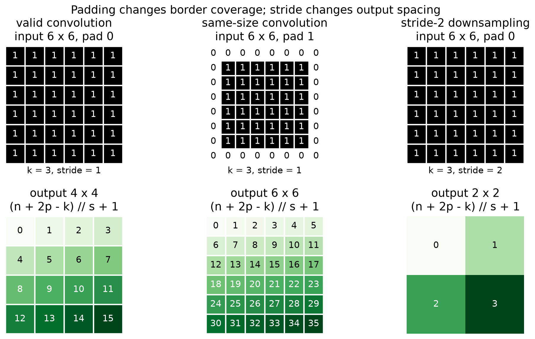
n_out = ⌊(n + 2·pad − k) / s⌋ + 1 — memorise this; you'll use it every time you sketch an architecture.Pooling — controlled downsampling
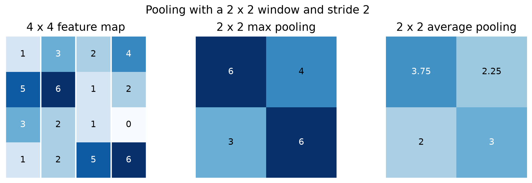
After each convolution, we typically halve the spatial dimensions with a pooling layer. Max pooling keeps the strongest activation in each window and discards the rest; average pooling smooths.
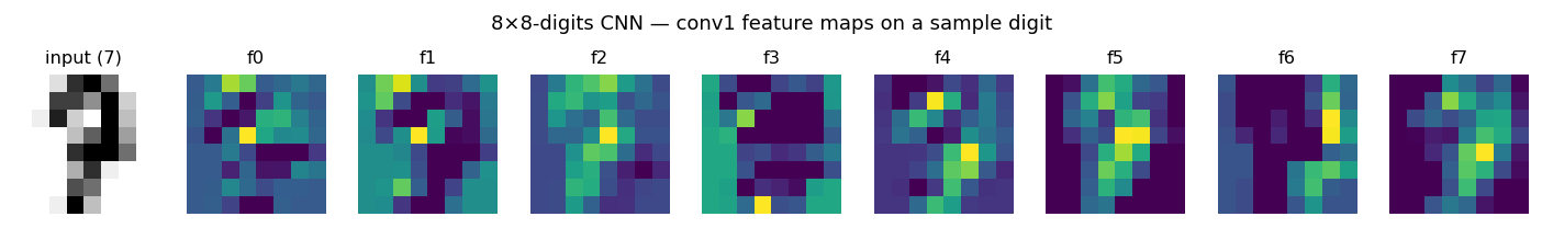
The trained CNN, opened up
CNNs are interpretable when they’re small. Each 3 × 3 filter in
conv1 ends up as an edge detector at some orientation, plus a few
blob/colour detectors. This is the same finding from the cat visual
cortex experiments that originally motivated CNNs.
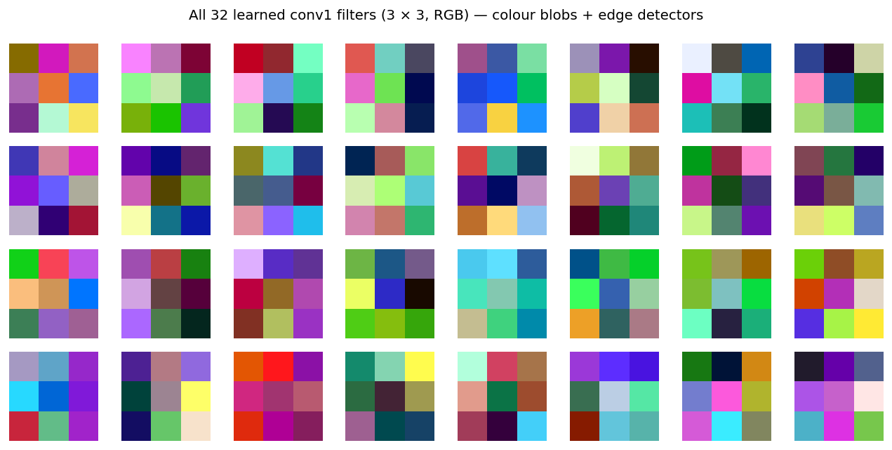
conv1 filters from the CIFAR-trained CNN. Each tile is a 3 × 3 × 3 RGB pattern. You can spot colour-blob detectors (uniform tiles), edge detectors (split tiles), and a few opponent-colour detectors.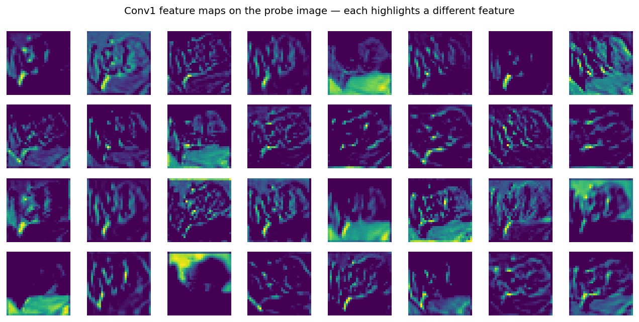
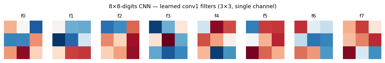
The notebook’s 8 × 8 digit version of the same interpretation:
What’s in here
- Why MLPs flatten the spatial structure of images and pay for it twice (lost locality + parameter explosion)
- The convolution operation with the output-size formula
- Padding, stride, and pooling — the three knobs every CNN turns
- A 2-conv-block CNN built in ~30 lines of PyTorch
- The interpretability story — learned filters as edge / colour detectors, feature maps as their responses
- Side-by-side MLP-vs-CNN training on CIFAR-10 with concrete parameter and accuracy numbers
- What changes for real-world datasets (batch norm, augmentation, pretrained backbones)
Prerequisites
- Tutorial 03 — the PyTorch training loop
- Comfort with image tensor shapes
[N, C, H, W]
Next
05 — Physics-Informed Neural Networks— what changes when the loss function knows physics, and how that opens up inverse problems and differentiable simulation.
References
- Hubel & Wiesel (1962). Receptive fields in the cat’s visual cortex. doi:10.1113/jphysiol.1962.sp006837
- LeCun et al. (1998). Gradient-based learning applied to document recognition (LeNet). doi:10.1109/5.726791
- Krizhevsky, Sutskever & Hinton (2012). ImageNet classification with deep CNNs (AlexNet). paper
- Zeiler & Fergus (2014). Visualizing and understanding convolutional networks. arXiv:1311.2901