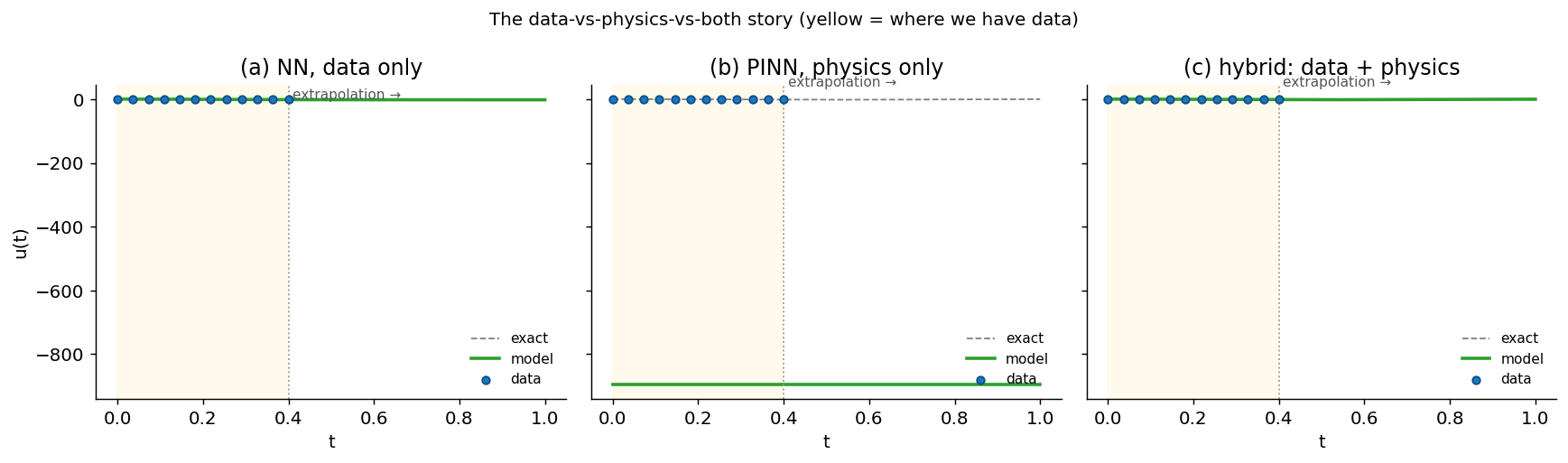
The failure mode that makes PINNs interesting is extrapolation. A plain neural network can fit the data you showed it and still become useless the moment you ask what happens next.
A PINN is a neural network with a physics term in the loss. That’s the whole idea. The rest is engineering: what to put in the loss, how to weight it, and why your first PINN will train to a flat function unless you do a few specific things.
# Track derivatives with respect to input time.
t = t.requires_grad_(True)

# Network prediction u(t).
u = model(t)

# First time derivative from autograd.
du_dt = torch.autograd.grad(u, t, torch.ones_like(u),
                            create_graph=True)[0]

# Second time derivative from autograd.
d2u_dt2 = torch.autograd.grad(du_dt, t, torch.ones_like(du_dt),
                              create_graph=True)[0]

# ODE residual for u'' + 2 zeta omega0 u' + omega0^2 u = 0.
residual = d2u_dt2 + 2 * zeta * omega0 * du_dt + omega0**2 * u

# Physics loss: make the residual small at collocation points.
physics_loss = (residual ** 2).mean()
The setup: pick a problem with a known exact solution, give yourself a small window of noisy data, then watch three models behave very differently when you ask them to predict the future. The damped-oscillator worked example below is directly inspired by Ben Moseley’s introductory PINN tutorial; the structure and core demo are his — go read the original.
Try it before you read it
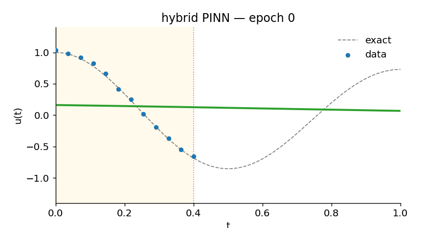
Slide through training epochs and watch the hybrid PINN find the oscillation. The yellow region is where it has data; everything to the right is extrapolation.
The setup
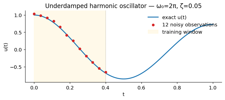
Light underdamped oscillator, \(\omega_0 = 2\pi\) (period 1, one full cycle in the window) and \(\zeta = 0.05\). 12 noisy observations in \(t \in [0, 0.4]\). The exact solution is a decaying cosine — which lets us measure error directly across the full window \(t \in [0, 1]\).
The extrapolation tax
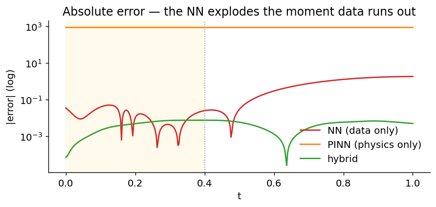
If you only care about one figure on this page, make it this one. Plain NNs diverge the moment the data runs out. Pure PINNs are stable but slow. Hybrid (data + physics) gives error a couple orders of magnitude lower than either, across the whole window.
Why does the data-only NN fail outside the training window? It is only penalised on \(t \in [0,0.4]\). Beyond that interval, the prediction is just the continuation implied by the learned weights and activation functions; there is no loss term telling it to obey the oscillator equation.
The physics loss changes that. Even where there are no observations, the network is penalised if \(u(t)\), \(u'(t)\), and \(u''(t)\) do not satisfy the ODE. It is still a neural approximation, but it is constrained by the differential equation rather than only by the observed data.
Watch the hybrid learn
What’s in here
- The damped-harmonic-oscillator ODE, with the exact solution for ground truth
- A 12-point noisy dataset that only covers the easy part of the trajectory
- Three models, same architecture: NN (data only), PINN (physics only), hybrid (data + physics)
- The
torch.autograd.gradrecipe for higher-order PDE residuals - Soft initial conditions, loss balancing, and the activation-function rule that bites everyone once
- A pointer at inverse problems — recover the unknown \(\omega_0\) and \(\zeta\) from the same 12 points
- A pointer at neural operators — what comes when one trained model needs to solve a family of problems
Why this matters for my own research
There is a clean inversion of the workflow you just did. We gave the network the equation and asked it to find the function. You can also give it the function (some experimental measurements) and ask it to find the equation — specifically, the coefficients of the equation.
Treat \(\omega_0\) and \(\zeta\) as torch.nn.Parameters and put them into
the optimiser alongside the network weights. PyTorch’s autograd will
backpropagate the data-loss gradient all the way through the physics
residual to those two parameters. This is called an inverse problem,
and it’s the engineering version of the “discover the laws of physics
from data” pitch.
This is the bridge between toy PINNs like this one and my own research
on torch_pf_solver
— a PyTorch fracture-mechanics solver where the unknown isn’t \(\omega_0\)
but the material toughness \(G_c\), recovered from a handful of
displacement observations of a real cracked specimen. The maths is
genuinely harder (the energy is non-convex, damage cannot heal, the
time-stepping is conditionally stable) but the autograd pattern is
literally what you wrote above.
Where to go after PINNs
A PINN trains one network for one problem. Change a coefficient or a geometry, you retrain. Neural operators learn the solution map — same model handles a whole family of inputs in milliseconds:
- DeepONet (Lu & Karniadakis, 2019)
- Fourier Neural Operator (FNO) (Li, Anandkumar et al., 2020)
- Siddhartha Mishra’s CIRM lecture series derives the theory from scratch — the recommended next watch after this tutorial.
Prerequisites
- Tutorial 03 — the PyTorch training loop
- Some familiarity with ODEs / PDEs — knowing what a damped oscillator describes is enough; PDE experience is a bonus, not required
References
- Raissi, Perdikaris & Karniadakis (2019). Physics-informed neural networks. J. Comp. Physics 378. doi:10.1016/j.jcp.2018.10.045
- Moseley (2021). So, what is a physics-informed neural network? benmoseley.blog — the tutorial this notebook’s damped-oscillator demo is built around.
- Krishnapriyan et al. (2021). Characterizing possible failure modes in PINNs. arXiv:2109.01050
- Lu, Jin et al. (2021). DeepONet. Nat Machine Intelligence 3. arXiv:1910.03193
- Mishra (2024). Learning operators — CIRM lecture series. YouTube — recommended next watch.
End of series
That’s all five tutorials. Back to the series →